arcgislayers is the core data access package in the R-ArcGIS Bridge, providing a unified interface for working with ArcGIS data services. As part of the arcgis metapackage, it enables seamless integration between R and the ArcGIS Web GIS ecosystem, including ArcGIS Online, Enterprise, and Location Platform.
An llms.txt file is available to provide context for LLMs when working with this package.
Capabilities
-
Connect to any ArcGIS Data Service: Access feature services, imagery, and portal items from ArcGIS Online, Enterprise and Location Platform using familiar R objects from
sfandterra. - Publish your R objects: Turn analysis outputs into live ArcGIS services that others can access, visualize, modify, and use in their workflows.
- Modify data in place: Maintain your production datasets—update, add, or delete features in feature services directly from R.
- Attachments: query, download, and update attachments in feature services created by Survey123.
Installation
arcgislayers is part of the arcgis metapackage, which provides the complete R-ArcGIS Bridge toolkit. For most users, installing the metapackage is recommended:
install.packages("arcgis")You can also install arcgislayers individually from CRAN:
install.packages("arcgislayers")To install the development version:
pak::pak("r-arcgis/arcgislayers")Usage
The basic workflow is: connect ➡️ query ➡️ analyze ➡️ publish. Here’s how to get started:
library(arcgis)
#> Attaching core arcgis packages:
#> → arcgisutils v0.6.0
#> → arcgislayers v0.6.1
#> → arcgisgeocode v0.4.0
#> → arcgisplaces v0.1.2
#> → arcpbf v0.2.0
Connect to ArcGIS Data Services
arc_open() connects to any ArcGIS data service using its URL or item ID. This creates a connection to the remote data without downloading anything yet.
# Connect to a feature service
furl <- "https://services.arcgis.com/P3ePLMYs2RVChkJx/ArcGIS/rest/services/USA_Counties_Generalized_Boundaries/FeatureServer/0"

county_fl <- arc_open(furl)
county_fl
#> <FeatureLayer>
#> Name: USA Counties - Generalized
#> Geometry Type: esriGeometryPolygon
#> CRS: 4326
#> Capabilities: Query,Extract
Query Data
arc_select() brings data from ArcGIS into R as familiar sf objects. You can get everything, or be selective:
# Get all data (use with caution on large datasets!)
counties_all <- arc_select(county_fl)

# Get specific columns and rows
large_counties <- arc_select(
  county_fl,
  fields = c("state_abbr", "population"),
  where = "population > 1000000"
)

large_counties
#> Simple feature collection with 49 features and 2 fields
#> Geometry type: POLYGON
#> Dimension:     XY
#> Bounding box:  xmin: -158.2674 ymin: 21.24986 xmax: -71.02671 ymax: 47.77552
#> Geodetic CRS:  WGS 84
#> First 10 features:
#>    STATE_ABBR POPULATION                       geometry
#> 1          OH    1264817 POLYGON ((-81.37707 41.3463...
#> 2          OH    1323807 POLYGON ((-83.24282 39.8044...
#> 3          PA    1250578 POLYGON ((-79.86399 40.2007...
#> 4          PA    1603797 POLYGON ((-75.1429 39.8816,...
#> 5          HI    1016508 POLYGON ((-157.6733 21.2980...
#> 6          IL    5275541 POLYGON ((-88.26711 41.9887...
#> 7          AZ    4420568 POLYGON ((-111.0425 33.4759...
#> 8          AZ    1043433 POLYGON ((-110.4522 31.7360...
#> 9          CA    1682353 POLYGON ((-121.4721 37.4777...
#> 10         CA    1165927 POLYGON ((-122.3076 37.8917...
Spatial and Attribute Filtering
Filter by location or attributes before bringing data into R:
# Spatial filter: get counties that intersect with North Carolina
nc <- sf::st_read(system.file("shape/nc.shp", package="sf"))
#> Reading layer `nc' from data source
#>   `/Users/josiahparry/Library/R/arm64/4.5/library/sf/shape/nc.shp'
#>   using driver `ESRI Shapefile'
#> Simple feature collection with 100 features and 14 fields
#> Geometry type: MULTIPOLYGON
#> Dimension:     XY
#> Bounding box:  xmin: -84.32385 ymin: 33.88199 xmax: -75.45698 ymax: 36.58965
#> Geodetic CRS:  NAD27

nc_area_counties <- arc_select(
  county_fl,
  filter_geom = sf::st_bbox(nc[1,])
)

nc_area_counties
#> Simple feature collection with 6 features and 12 fields
#> Geometry type: POLYGON
#> Dimension:     XY
#> Bounding box:  xmin: -82.0477 ymin: 35.98946 xmax: -80.83795 ymax: 36.80746
#> Geodetic CRS:  WGS 84
#>   OBJECTID             NAME     STATE_NAME STATE_FIPS  FIPS     SQMI POPULATION
#> 1      467   Johnson County      Tennessee         47 47091 302.6644      17948
#> 2     1924 Alleghany County North Carolina         37 37005 236.1822      10888
#> 3     1926      Ashe County North Carolina         37 37009 429.3538      26577
#> 4     2016   Watauga County North Carolina         37 37189 313.3604      54086
#> 5     2018    Wilkes County North Carolina         37 37193 756.5252      65969
#> 6     2995   Grayson County       Virginia         51 51077 445.7267      15333
#>   POP_SQMI STATE_ABBR COUNTY_FIPS Shape__Area Shape__Length
#> 1     59.3         TN         091  0.07960385      1.290607
#> 2     46.1         NC         005  0.06140165      1.231232
#> 3     61.9         NC         009  0.11428581      1.442112
#> 4    172.6         NC         189  0.08142272      1.287674
#> 5     87.2         NC         193  0.19911944      1.984232
#> 6     34.4         VA         077  0.11578917      1.945424
#>                         geometry
#> 1 POLYGON ((-81.74091 36.3919...
#> 2 POLYGON ((-81.2397 36.36549...
#> 3 POLYGON ((-81.47258 36.2344...
#> 4 POLYGON ((-81.80605 36.1046...
#> 5 POLYGON ((-81.02037 36.0350...
#> 6 POLYGON ((-81.34512 36.5729...
Use list_fields() to explore available attributes:
list_fields(county_fl)
#> # A data frame: 12 × 10
#>    name         type  alias sqlType nullable editable domain defaultValue length
#>  * <chr>        <chr> <chr> <chr>   <lgl>    <lgl>    <lgl>  <lgl>         <int>
#>  1 OBJECTID     esri… OBJE… sqlTyp… FALSE    FALSE    NA     NA               NA
#>  2 NAME         esri… Name  sqlTyp… TRUE     TRUE     NA     NA               50
#>  3 STATE_NAME   esri… Stat… sqlTyp… TRUE     TRUE     NA     NA               20
#>  4 STATE_FIPS   esri… Stat… sqlTyp… TRUE     TRUE     NA     NA                2
#>  5 FIPS         esri… FIPS  sqlTyp… TRUE     TRUE     NA     NA                5
#>  6 SQMI         esri… Area… sqlTyp… TRUE     TRUE     NA     NA               NA
#>  7 POPULATION   esri… 2020… sqlTyp… TRUE     TRUE     NA     NA               NA
#>  8 POP_SQMI     esri… Peop… sqlTyp… TRUE     TRUE     NA     NA               NA
#>  9 STATE_ABBR   esri… Stat… sqlTyp… TRUE     TRUE     NA     NA                2
#> 10 COUNTY_FIPS  esri… Coun… sqlTyp… TRUE     TRUE     NA     NA                3
#> 11 Shape__Area  esri… Shap… sqlTyp… TRUE     FALSE    NA     NA               NA
#> 12 Shape__Leng… esri… Shap… sqlTyp… TRUE     FALSE    NA     NA               NA
#> # ℹ 1 more variable: description <chr>
Work with Imagery
arc_raster() extracts raster data from ArcGIS ImageServers as terra objects:
# Connect to Landsat imagery
img_url <- "https://landsat2.arcgis.com/arcgis/rest/services/Landsat/MS/ImageServer"
landsat <- arc_open(img_url)

# Extract imagery for a specific area
res <- arc_raster(
  landsat,
  xmin = -71,
  ymin = 43,
  xmax = -67,
  ymax = 47.5,
  bbox_crs = 4326,
  width = 250,
  height = 250,
)

terra::plot(res)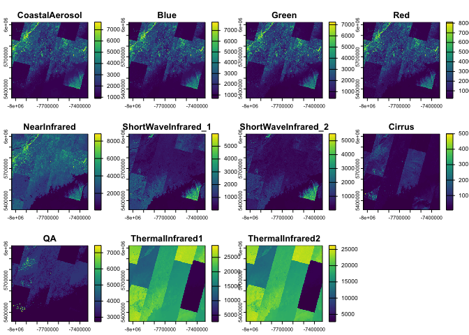
Publish Your Results
Turn your R analysis into ArcGIS services that others can access:
# Publish an sf object as a feature service (requires authentication)
my_analysis <- large_counties |>
  dplyr::mutate(density_category = ifelse(pop_sqmi > 100, "Dense", "Sparse"))

publish_layer(
  my_analysis,
  title = "County Population Density Analysis",
  description = "Counties categorized by population density"
)
Learn more
To learn more about about how to most effectively use arcgislayers for your use case review the developer site documentation.